The Segregation Model
- Source Code and Java Documentation (729 KB)
- Java Documentation
-
Data sets (2.76 MB)
The following page will introduce the reader to the basic segregation model developed for this paper. The inner workings of the conceptual model will be presented. The model, as with all abstractions, tries to build a representation of the real-world, making choices about what to represent and at what level of detail. For this reason, the methods within the model are totally flexible, as in the basic model, there is no hard coding of geometries and the model itself can easily be extended to examine different aspects of segregation phenomena. The sorce code for the model can be downloaded from here.
As with Schelling’s (1971) original model, the basic segregation model has two types of agents, and for simplicity, these will be called red and blue. However, they could be considered as two racial groups or households or firms etc. Each agent has a specific spatial location and can calculate its neighbourhood composition (see below) and it only moves (see evaluateAndSetHappiness method in Resident class) when it is dissatisfied with this current neighbourhood composition. All the individual agents within each group will have the same preference for neighbourhood configurations. All the agents are located within the urban environment which acts as a container for agents (see below). Figure 1 highlights the basic properties of an agent, in this example, it is a red agent. These properties include its location (see getLatLon method), its satisfaction for its current neighbourhood (see getHappyness), social class (see getSoc method), and the number of times it has moved (see getNumberOfTimesMoved). Additionally the aggregate proprieties of the system are recorded by the environment, specifically, its predominant social class (see socialClassOfUrbanAgent method in Urban Agent class) which in this case is mixed as there are equal numbers of red and blue agents. Its population relates to the number of agents that fall within its boundary and its area.
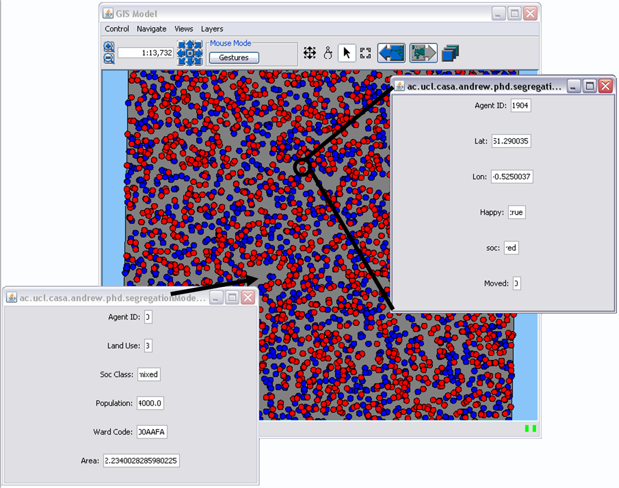
Figure 1: Basic properties of a red agent and the underling environment.
Figure 2highlights the user interface of the model. Clockwise from the top left is the control bar for the simulation, the GIS display which shows the agents and the urban environment which in this case are the wards of the City of London, graphs for aggregate outputs, a legend for interpretation of the GIS interface, model output in the form of text, and the model parameters.
Figure 2: Segregation model user interface (showing segregation dimensioned to the geography of wards in the City of London).
Neighbourhood Calculations
It is the agents’ neighbourhood which drives the process of segregation. As with other segregation models, the model assumes that agents want to live with those who are of similar type to themselves. Therefore individuals exhibit a threshold in their preferences for a certain neighbourhood racial composition. As the model is vector-based, it does not use cells neighbouring the agent to calculate neighbourhoods; instead neighbourhoods are established by creating a buffer at a specified radius around the agent in question and then calculating how many agents and of what type are within the buffer (Figure 3) taking into consideration geographical features (see basic model and neigboursWithin method in resident class). If the agent is dissatisfied with its current neighbourhood configuration, it will move to a new area where its preferences are met.
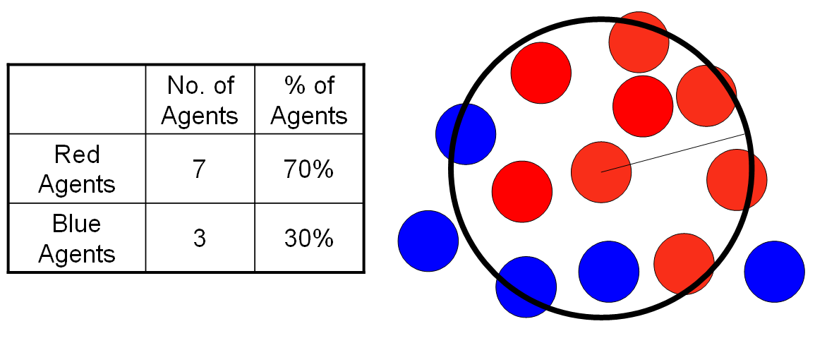
Figure 3: An agent evaluating its neighbourhood at a specific radius.
Movement
At each time step within the model (see step method in Resident agent class for further details), every agent evaluates its neighbourhood and has the ability to move if it is dissatisfied with its current neighbourhood configuration (see evaluateAndSetHappiness method in Resident class). As with Schelling’s (1971) original model, time within the model is purely abstract, but a more detailed model however could be developed to allow the agents to move at specific time intervals. This was not considered important in this model as the focus was on the way patterns emerge and dissipate over time.
Similar to Schelling's original model, the agent moves to the nearest area where its preferences will be satisfied. This assumption is also supported by empirical evidence for the Greater London Authority (GLA) which showed that the largest borough to borough flows are moves to adjacent boroughs (Mackintosh, 2005). An agent’s movement is accomplished by first randomly searching its initial area for a neighbourhood where it will be satisfied. If after searching its immediate area 25 times (the number 25 was chosen as the agent could continuously search its area randomly or focus it on a specific area for simulation speed), the agent is still dissatisfied, a second searching mechanism is used in that the agent will then move to its nearest neighbour of the same type which is satisfied with its current position (measured using Euclidian distance) from where the agent was originally placed. Unlike calculating neighbourhoods, movement is not restricted by geographical features. Once the agent has moved to its nearest neighbour, it carries out a local search around that agent’s neighbourhood for a suitable location (Figure 4 and moveAgentUntilHappy method in Resident class). Each time the agent moves to a new position, it creates a buffer evaluating its immediate neighbours. If the agent cannot find a suitable location at this point, it then moves to the next nearest agent of the same type and searches that area and so forth until it finds an area it is satisfied with. If the agent cannot become satisfied within the environment, it leaves the system altogether. This removal of agents is unlike that in Schelling’s model. It was incorporated into this model as unlike Schelling’s model, no space is given to empty cells. Figure 5 highlights this searching mechanism. It needs to be stressed that as the model is based on the vector representation of space, both the random and local searching is not restricted to discrete cells, as the model does not use cells to divide the space.
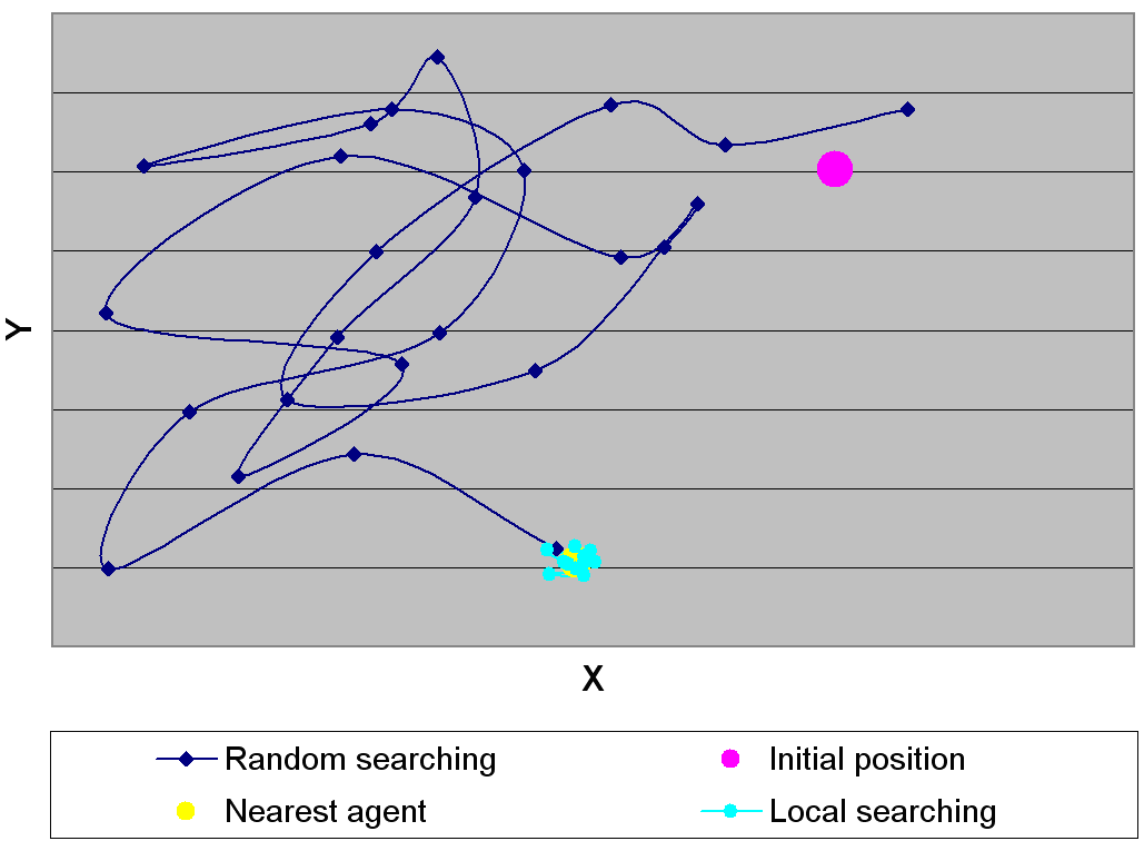
Figure 4: An example of searching for one point agent. From the initial location, this shows the random search path before moving to its nearest neighbour and carrying out a local search.
Figure 5: Movement of point agents within the basic segregation model through one time step.
The Agents and the Environment
The model is comprised of residential agents who are located within an environment. The agents are extensions of the basic point agent class and the environment extends the basic polygon agent class. It is the actions of these agents that will create changes in the physical environment. The model builds agents based on population data held within fields of the shapefile which represent the urban environment (see Basic Model). This could be considered as population counts from census data at a specific geographical scale, for example, a ward. The shapefile also acts as the artificial world in which the agents interact with each other. As the agents move about the system, the environment changes and thus the predominant social group in the area might change. Figure 6 highlights how this change may occur by agents moving from one area to another over a period of time. The underlying ward colour relates to the predominant social group of the area. Additionally the environment maintains aggregate information such as population counts (which are updated at the end of each time step, once all the agents have had the option to move, see socialClassOfUrbanAgent method in Urban Agent clas).
Figure 6: Changes in the makeup of an area over time.
Steps within the Segregation Model
The following subsection will outline the basic processes within the segregation model. Figure 7 sketches out the main processes within the model. Once the model is first initialised, the vector GIS data is read into the model and used to build the residential/point agents (see buildModel method in SegGISModel). Once the agents have been created, the displays are then built (see buildDisplay method in SegGISModel). However, before entering the run phase of the model, events are scheduled to take place at specific periods throughout the simulation (see buildSchedule method in SegGISModel). The order which events are scheduled is first pre-Step (see preStep method in SegGISModel) where the environment and agent characteristics are updated if changed by the user.
Secondly Step is called(see step method in SegGISModel). Within Step, each agent has the option to move where movement is governed by an agent evaluating its neighbourhood and if dissatisfied with its current neighbourhood configuration, the agent moves (as described above). If the agent moves, a counter is used record this movement. Once all the agents have had the option to move, post-Step is called (see postStep method in SegGISModel). Within post-Step, the residents evaluate their neighbourhoods (see evaluateAndSetHappiness method in Resident class). As agents only move to areas where their preferences are satisfied, one might expect all agents to be satisfied with their current surroundings. However, the movement of other agents during the course of one time step will affect other agents within the system; thus it is useful to keep track of how many agents are currently satisfied. Additionally in post-Step the environment updates its characteristics based on what types of agents are within it. This updating of agents is then recorded to new shapefiles, one for the agents’ locations and one pertaining to the environment (e.g. how many agents and of what type are within a ward). Aggregate information such as the total number of agents dissatisfied is outputted to a text file. Additionally, this information is used to update the displays of the model. Once this has been done, the model then moves back to pre-Step. The model continues to run until all agents are satisfied with their neighbourhood configuration or is stopped by the user.
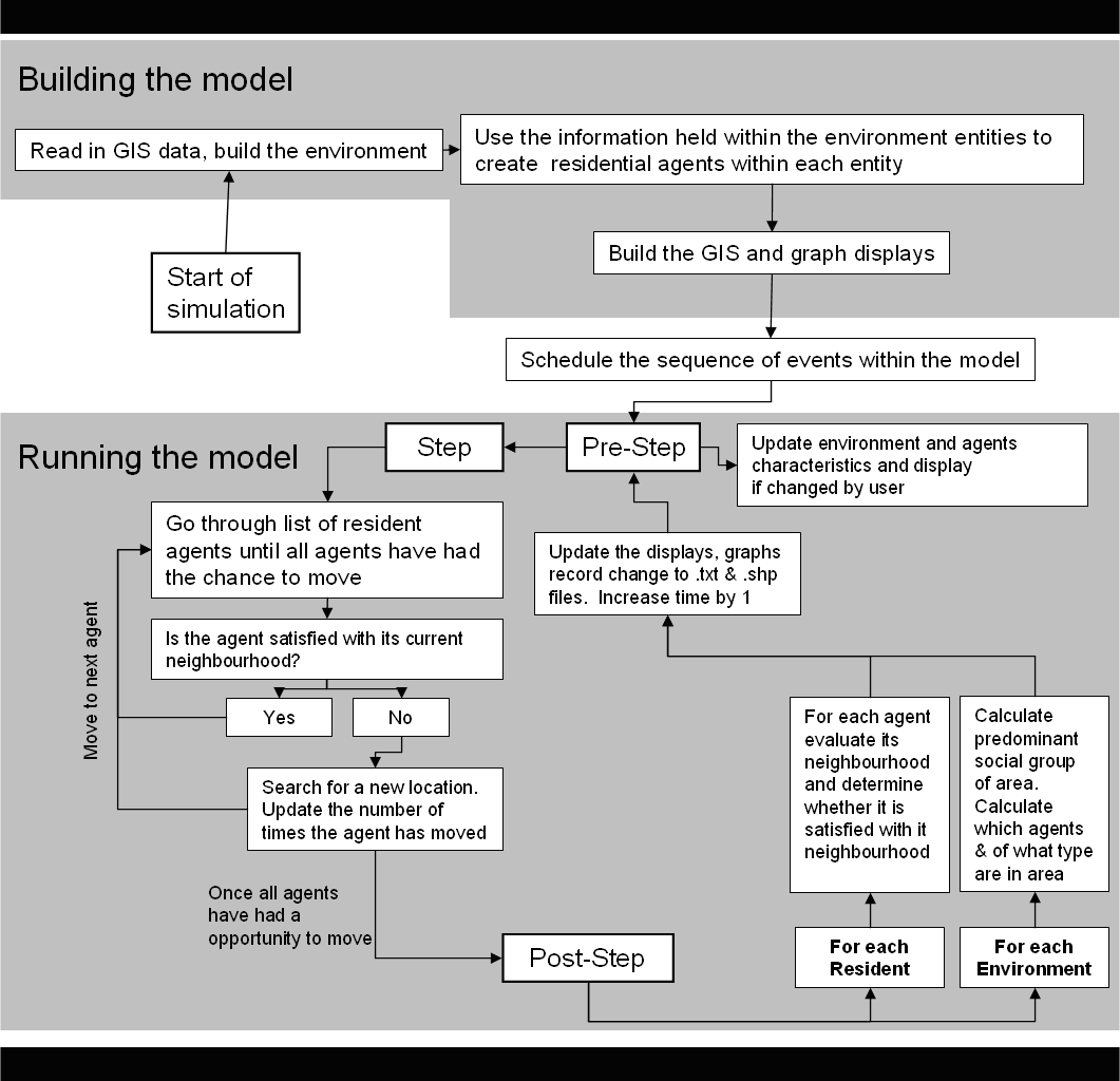
Figure 7: Flow diagram of the key process within the segregation model.
References
Mackintosh, M. (2005), Data Management and Analysis Group Briefing 2005/30: 2001 Census: The Migration Patterns of London’s Ethnic Groups, Greater London Authority, London, UK.
http://www.london.gov.uk/gla/publications/factsandfigures/dmag-briefing-2005-30.pdf.
Schelling, T.C. (1971), 'Dynamic Models of Segregation', Journal of Mathematical Sociology 1: 143-186.