The Basic Model
- Source Code and Java Documentation (728 KB)
- Java Documentation
- Data sets (2.20 MB)
The basic model was written in Java, which is a fully object-orientated programming language and extends a number of basic operating classes from the Repast library. While Repast provides a basis for creating models, the modeller needs to design/encode rules for agent interaction thus making the model context-specific. Within the model, Repast is primarily used for its display, scheduling, and importing GIS vector data (ESRI shapefiles) though its interface with the GeoTools library along with recording change classes, specifically outputting data as new shapefiles. The program utilizes other Java-based GIS libraries especially those from the JTS which provide general 2D spatial analysis functions such as line intersection algorithms and buffering, and OpenMap which provides a simple GIS display with panning and zooming and querying of the GIS layers. One could have used ArcGIS for the display of the simulations through Agent Analyst. However, this has limitations when it comes to developing and running the model on computers that do not have ArcGIS installed. What the basic model does is to link these various components together to form a geographically explicit agent-based model.
The initial aim was to develop as much functionality as possible into a basic spatial ABM application which could then be applied and extended to explore a range of urban models, utilizing the Repast framework, specifically its support of vector GIS integration. The following subsections provide details of the model with the actual source code and demos etc. can be found here.
Building the Model: Data Representation
The world is infinitely complex, and one needs be able to abstract key features and build a representation of those features. The basic model was designed to work on many different geographical scales (e.g. boroughs, wards, output areas, and MasterMap TOIDs) without the need for model reconfiguration (Figure 1). Therefore any vector shapefile projected in World Geodetic System 84 can be used as a representation of the environment under investigation. This was considered important as most socio-economic data comes in this format, for example, census and geo-demographic data. This was accomplished by extending Repast’s ability to read in shapefiles by creating a set of methods which read in the geometry of the shapefile and build the appropriate dataset, rather than hard-coding individual dataset geometries. This functionality was created as all too often models are applied to one specific geographical area and not another. The ability to create a model for one area and then apply it to another area allows the modeller to see if the same rules can be applied to different areas and at different scales.
Once the environment has been chosen, the actor/agents need to be created. Within the model, there are broadly two types of agents possible; animate (non-fixed) and inanimate (fixed) agents. Each agent type can be can be seen as similar to a layer in a GIS, and each agent in a model is similar to a feature in a GIS (Najlis and North, 2004). The model uses attribute data from the polygon shapefile, i.e. from the .dbf file to create agents. Agents can either be the polygons themselves and are classed as inanimate as they do not actually move, for example, land parcels (see The Polygon Agents section), or points which can be inanimate or animate directly positioned on top of the polygon layer, for example, residents located within the urban environment (see the Point Agents section).
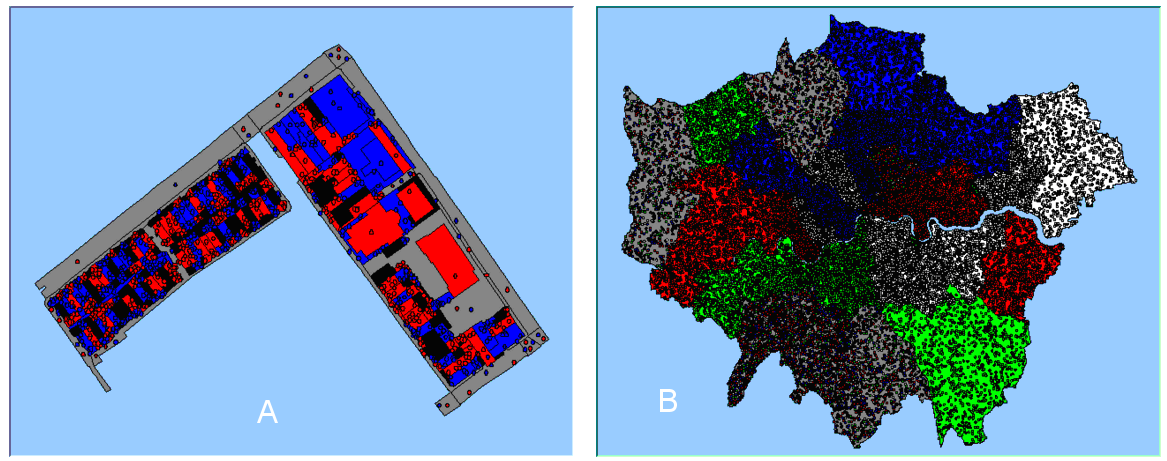
Figure 1: Spatial representation within the model. A: street section composed of MasterMap TOIDS. B: London composed of boroughs. Agents are shown as dots.
The inanimate agents are created using Repast’s built in functionality, specifically, by reading in the shapefile, related to the specific area of interest. The data are held in a table across several columns or fields. Each table row is a record, and each row becomes a polygon agent. For the creation of point agents, there are several fields associated with each row and the correct numbers of agents are therefore created. To illustrate this process, take for example, an area with four wards (Figure 2A); all the wards have attribute data associated with them stored in a table, with several fields and rows. Each row relates to a specific ward. For instance ward 1 has a population of 10 red, 5 blue, 4 green and 2 white. The model reads in this data and creates an agent for each ward and the desired population based on data held in the fields (Figure 2B). The underlying ward colour represents the predominate social group of the area. All these features can be seen in the build model method of the model.
Figure 2: Reading in the data and creating the agents.
Point agents (e.g. residents) are placed randomly throughout the polygon agent, due to our ignorance over knowing exactly where they are located due to the aggregated nature of the data. Most datasets are based on aggregated data, due to the availability of personal data being regulated by laws (data privacy regulations in Europe, for example). In some cases, privacy limitations and the demands of the research are contradictory, for example, in building populations of individuals within an agent-based model. The solution this research takes is building a synthetic population. Such data imitate statistical properties of the investigated population. The population parameters are usually easily available just because the aggregate data are sufficient to estimate them. This is a similar approach to that of microsimulation models such as TRANSIMS model applied to Portland where Barrett et al. (2001) generated a realistic-looking and statistically robust population data at the micro-scale. Synthetic households were generated with demographic and socioeconomic attributes geo-referenced to micro-scale geographies. The results generated on this basis are like the original data, but without sacrificing the privacy of urban residents.
The ability to model actual decision making units such as the individual, the household, and the firm allows one to build on the growing knowledge of how individuals interact to form aggregative outcomes which are all too familiar when examining the city. It is believed that this approach to modelling will facilitate and improve our ability to test behaviours about individuals and how these individual decisions lead to improving our predictions about aggregative aspects of our socio-economic system. Therefore the creation of artificial populations of point agents moves away from the aggregate counts which suggest uniformity at the aggregate level. Additionally, the ability to create agent descriptions based on data about the area allows for the setting of the initial starting conditions of the model, for example, land-use or the predominant social class of the area.
While point agents are placed randomly within the area, a model could be built that would place agents in a precise location if high resolution geographic databases of population were available (see Adding Extra Layers section for an example). For example Ordnance Survey’s MasterMap dataset for roads, houses etc could be combined with UK census data. An example of this approach is that of Benenson and Omer (2003) who examined 1995 individual census data from the Israeli Central Bureau of Statistics with Benenson et al. (2002) using this data to calibrate an agent-based model.
The Polygon Agents
Essentially, the polygon agents form the environment of the model and can represent a diverse range of areas from houses to wards. These can either be agents in their own right or just containers of the point agents. In both instances, the polygon agent also contains aggregate information pertaining to features within it. These could include, for example, number and type of various point agents (though point in polygon operations) and thus give the population density of an area. This is achieved because each polygon agent contains geometrical information about itself, for example, a list of coordinates which makes up its’ extent and the centroid of the polygon. This information can be used to calculate distances between polygons if needed. Additionally any information from the polygon attribute file (.dbf) can be included in the agent description, for example, whether it is a park or a housing estate. In a sense, polygon agents can be considered as irregular cells and can work in a similar way to cell space models where the cells remain fixed but can change their state. This can be achieved by the polygon agent ‘knowing’ its neighbours.
Neighbourhoods are calculated using Repast’s inbuilt readNeighborhoodInfo method which requires a .GAL (GenePix Array List.) file. This is not to say it cannot be done using JTS, but it is done this way to speed up the execution of the model as it provides an easy way to link between location and the quantitative values that represent each polygon. Basically, a .GAL file is a text file with specific information and used within the program to create an array list. They are easily created using Visual Basic in ArcGIS or using GeoDa, a freely downloadable program designed to implement techniques for exploratory spatial data analysis on lattice data (points and polygons). The .GAL file contains information about the number of polygons within the shapefile (Figure 3). In the case below, it is 0 to 6 (the last polygon in the list), the file name (all_data_small) and the column name (ID_ID) where the polygon identifier can be found (Figure 3). When the model is first initialised, the polygon shapefile is read in; this in turn calls the .GAL file and links the data pertaining to the polygon agent’s neighbours with the attributes of the polygon (see Segregation Polygon Model for an example).
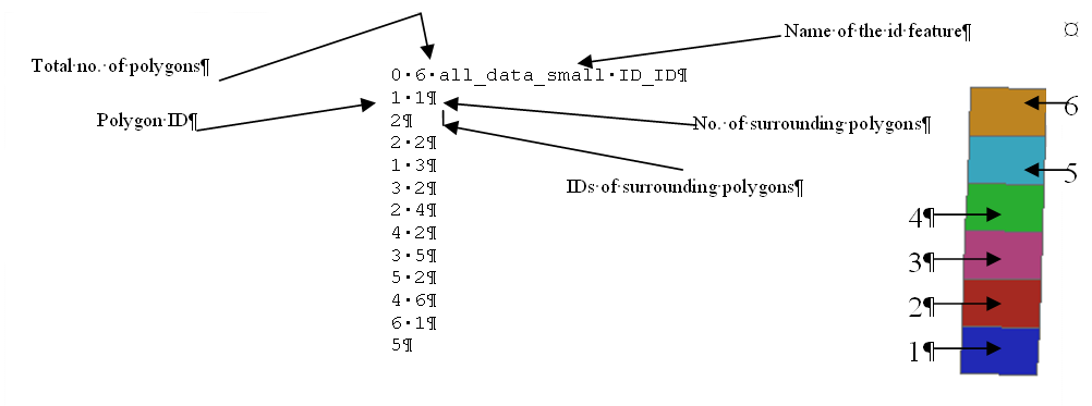
Figure 3: Annotated example of a .GAL file and the associated shapefile with the polygons numbered accordingly.
[TOP]Adding Extra Layers
As the model uses a vector approach to representing space, both points and lines (See BasicPoint and BasicLine respectively) can additionally be represented within the model as extra layers. These can either be loaded through the use of a shapefile or created on the fly for the case of point agents described above. The ability to add features apart from polygons allows for different features such as underground stations or train lines to be incorporated into the model if desired. If one had the exact residence of each person, these could therefore be added to the model. The point agents can then interact with these features if needed. For example, when choosing a new house, a residential agent may consider distance to the underground station or the agent may not want to live next to main road. Figure 4 demonstrates how different layers can be added to the model, the underlying environment layer (the red polygons) representing wards, on top of which point agents were created based on attributes of the .dbf file (as described above). Additionally two extra layers have also been added, one of lines and one of points based on a line and point shapefile respectively. The points (white points) represent the location of actual underground stations while the black lines connecting the underground stations represent the underground lines in this central London example.
Figure 4: A screen shot where extra layers have been added
The Point Agents
While the polygon agents remain fixed, the point agents can either be inanimate/fixed (such as underground stations) or animate/mobile (such as residents). Both are located within the urban environment and are capable of interacting with each other and the environment. As with the polygon agents, this type of agent is built with flexibility in mind, for all modellers try to build a representation of the real-world, making choices, about what to represent and at what level of detail. Modellers are therefore faced with the challenge of abstraction. Agent-based models focus on the individual with individual characteristics located in space whose behaviour has to be described over time. The modeller has therefore to make decisions about these issues specifically in terms of: sectors (number and breadth of categories, e.g. splitting the population by age groups), space (size of area units within which entities are located, e.g. a census track), and time (length of time units which provide the basis for longitudinal description and analysis e.g. 10 year time intervals) (Wilson, 2000). For this reason, the point agents’ characteristics are totally unspecified. Specification comes when designing the specific application.
While the point agent’s characteristics are unspecified, there is some core behaviour. Specifically the agent needs to know where it is and which agents are surrounding it; additionally methods are needed for the movement of agents. Two types of movement are built into the model for point agents. One is the movement between areas, for example, between wards, and the second is local movement. Movement between areas can be carried out in two ways. One is by searching an area’s aggregate characteristics and deciding if it is suitable for the agent. Secondly it can be facilitated by the agent’s preferences for other agents, for example, moving to an area due to similar agents already located there (as in the case in the Segregation Model). In either case, once an agent moves to a new location, there are a series of methods for local movement.
Unlike in pedestrian modelling, the agent’s movement is not dictated by a specific target. Local movement within the model is focused on allowing the agent to search its local environment to see if a suitable location can be found. Agents do not just move between polygons but also within them which distinguishes them from cell space models. This movement can be constrained to a specific area, for example, a ward, and the distance between points can be specified. However, the movement itself is random (Figure 5 or agentMovesToNewLocation method in BaiscPointAgent for an example). Each time the point agent moves, a buffering operation (see below) can be carried out to determine the local neighbourhood characteristics (Figure 6 or summaryOfNeibourhingAgents method in BaiscPointAgent for an example). It is worth noting that the buffered areas appear ellipsoid in shape which is a result of transforming the coordinates from WGS84 to a projected coordinate system/flat surface. This effect will be seen throughout the paper where coordinates have been taken directly from the models and projected to a flat surface but it makes no difference to the underlying locational frame which remains accurate. It is simply an artefact of the simulation and could be corrected deep within the basic code.
Figure 5: An example of pseudo random movement of a agent searching
Figure 6: Agents' movement in red and their buffers in black; the buffer centroid is based on the agents' centroid.
GIS Operations
The ability to represent the urban system as a series of spatial objects – points, lines and polygons each with a spatial reference describing the location of the object rather than just as a series of cells, leads to conceptual problems such as defining neighbourhoods, new searching algorithms, and movement rules. To overcome these problems, the model relies on a series of spatial analysis operations. The following section introduces the operations most commonly used within the model specifically, buffering and union.
Unlike that of cellular space models where neighbourhoods are often calculated using Moore or von Neumann neighbourhoods or variations, the use of irregular cells (polygons) and points mean different tools are needed to calculate neighbourhoods. Two different neighbourhood mechanisms are used within the model, one for polygons and one for points. Both mechanisms allow for the treatment of physical boundaries (e.g. rivers and motorways) to be incorporated into the model.
Polygon neighbourhoods are defined as those polygons which share an edge with another polygon agent (adjacency) through the use of .GAL files (see above). For point agents, buffers are created. Using a vector space, buffers are often used to calculate neighbourhoods. This involves the creation of a circular region around a point, or a corridor around a line feature. The radius of the circle or the width of the corridor is defined by the analyst usually using Euclidian distance. Buffers are often used in GIS to reflect notions of accessibility or proximity to geographical features.
Figure 7 highlights how a geographical feature (such as a river) can be incorporated into the model when calculating neighbourhoods. Within Figure 7, the black circle represents the point agent of interest. This agent wants to know which agents are within a specified distance of itself and in the same geographical area. A buffer is created at this specified distance based on the centroid of the agent. However, in this case, the buffer crosses the river. Therefore agents on the other side of the river (yellow squares) are not neighbours as there is no way for them to move directly to the agent; however, they are within the buffered region (green line). Those agents (red squares) which are on the same side of the river as the agent and are within the agents’ defined buffer (red line) are classed as neighbours, and any agents outside this area would not be classed as neighbours. This creation of buffers also has the advantage of calculating local statistics such as population density of small areas etc. However, if there was a bridge connecting the two areas, the agents on the other side of the river would be considered neighbours (Figure 8).
Figure 7: Defining neighbourhoods with the inclusion of geographical features (constrained buffer)
Figure 8: Defining neighbourhoods with the inclusion of geographical features where the two areas are connected by a bridge.
Agent-based models create worlds populated by agents where these agents are free to explore this world. However, such worlds often have boundaries. Within a cellular world, this is based on the matrix of cells, for example, a 10x10 regular lattice of cells, say. However, as one moves to a representation of space using irregular cells, this is no longer the case. One has to define the boundary of this world. To accomplish this task, the model uses the spatial analysis operation known as union. Simply stated, union combines the polygons and returns one extent of the whole area. This is then used as the boundary for the model. Figure 9 highlights how individual borough boundaries (black lines) are combined to form a boundary (red line) which retains the original geometry and restricts agents’ movement to within it. For the actual code see the getUnion method in BasicPolygonAgent class.
Figure 9: The union of individual polygons to form a boundary for the model.
As each agent class is represented as a separate layer, one needs to relate objects in one layer to objects in another. This is achieved through a point in polygon analysis. This allows the model to determine whether a given point lies inside a specific polygon. The ability to carry out point in polygon operations, for example, the number of point agents that are contained within a polygon, allows the model to be generative. In this sense, entities at higher levels of geographic representation such as population counts are derived from the bottom-up, through interactive dynamics of collections of animate objects observed at the micro-scale.
The GIS operations that have been described in this section allow an agent-based model to be created where space and geometrical relationships are explicitly incorporated into the simulation. Each type of agent knows its position and can use the operations such as buffering and point in polygon to find out more about its neighbourhood.
Recording Change
The recording and visualisation of change is of great importance to ABM. It allows the user to see change occurring within the model as it happens and also helps with analysing the model outcome. The basic model uses Repasts inbuilt functions for the recording of change during the simulation run. These include graphing options, screen capture, the creation of movies, and aggregate information in the form of text files, along with the creation of new Shapefiles of both polygon and vector agents (Figure 10). The latter allows for spatial analysis after the model simulation has been run, whilst at the same time keeping track of changes in between time steps within the model, for instance changes in population density within the environment as agents move into and out off an area. This recording of change at a higher, aggregate level as well as at the individual agent level, allows one to see how micro change affects higher level viewing. Expample methods are setSnapShotRecording and saveShapefile methods in the BasicModel class
The recording and visualisation of change is of great importance to ABM. It allows the user to see change occurring within the model as it happens and also helps with analysing the model outcome thus facilitating verification of the model. The basic model uses Repast’s inbuilt functions for the recording of change during the simulation run. These include graphing options, screen capture, the creation of movies, and aggregate information in the form of text files, along with the creation of new shapefiles of both polygon and point agents (Figure 10). The latter allows for spatial analysis after the model simulation has been run, whilst at the same time keeping track of changes in between time steps within the model; for instance, changes in population density within the environment as agents move into and out of an area. This recording of change at a higher, aggregate level as well as at the individual agent level, allows one to see how micro change affects higher level aggregation and the resultant patterns. Expample methods are setSnapShotRecording and saveShapefile methods in the BasicModel class.
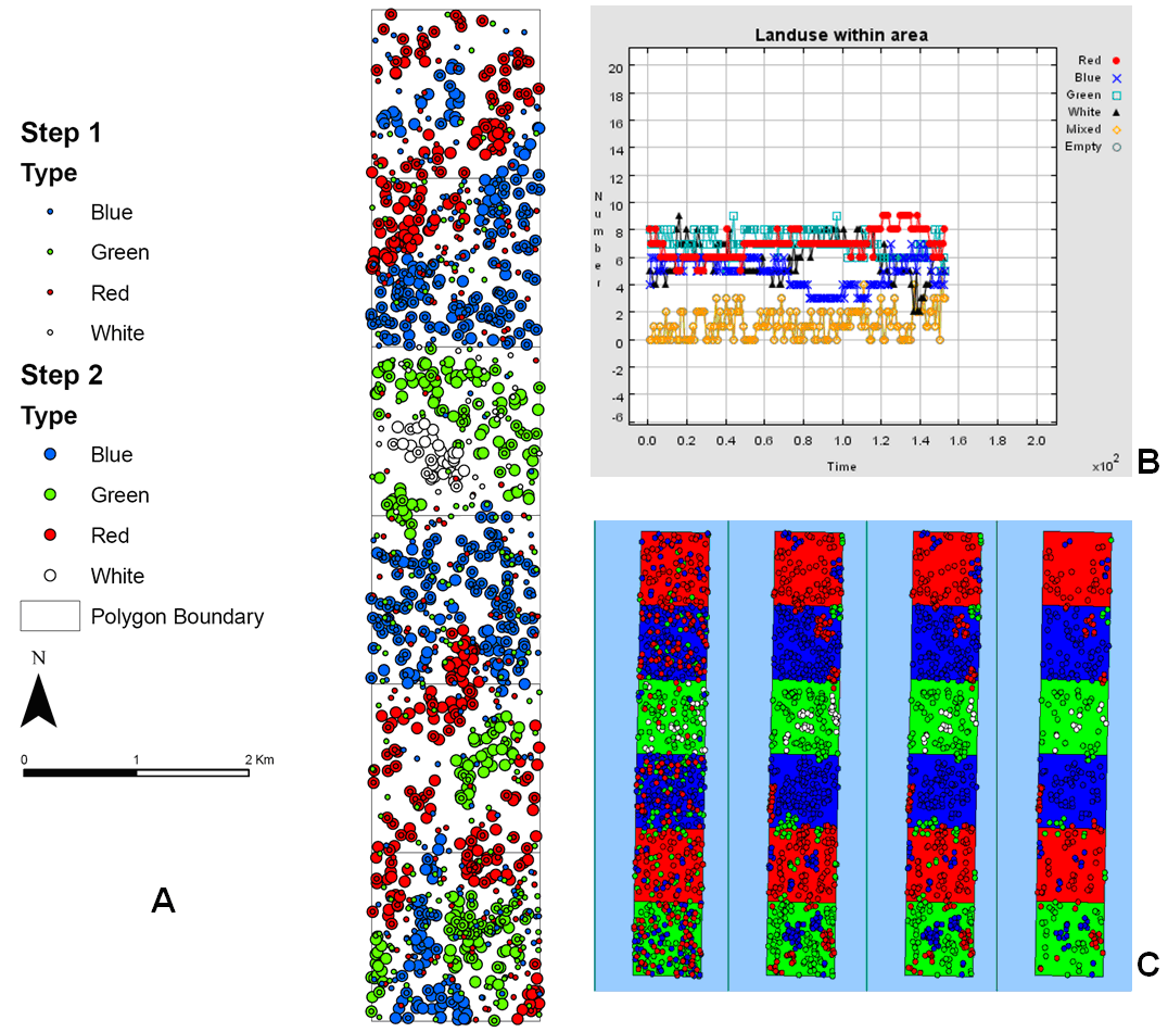
Figure 10: Examples of the different types of outputs from the model. A: point shapefiles of locations of point agents in two different time steps (step 2 are the larger circles), B: graph showing land-use change during a model run, C: series of screen captures.
User Interaction
As the models are based on the concept of a tool to ‘think with’, user interaction is key as it allows for the model to be open. User interaction is in the form of parameter settings, the movement of agents via drag and drop, and the ability to change the agent attributes, all via a GUI which allows for sensitivity testing of model ‘Parameters’. Figure 11 highlights how the user can set model parameters at the start and during the simulation run. Additional information about the model can also be provided by choosing the ‘About this model’ button (Figure 12A) which opens up a new window which the user can scroll through and read about the basic structure of the model, what each of buttons are designed to do etc. (Figure 12B). Also included on the ‘Custom Actions’ panel is a ‘Simulation Speed’ slider which slows or speeds up the program. Sometimes it may run too fast to see exactly what is changing and needs to be slowed down. Both of which are set in the setup method of the BasicModel.
Figure 11: An example of 'Parameter' settings for the model.
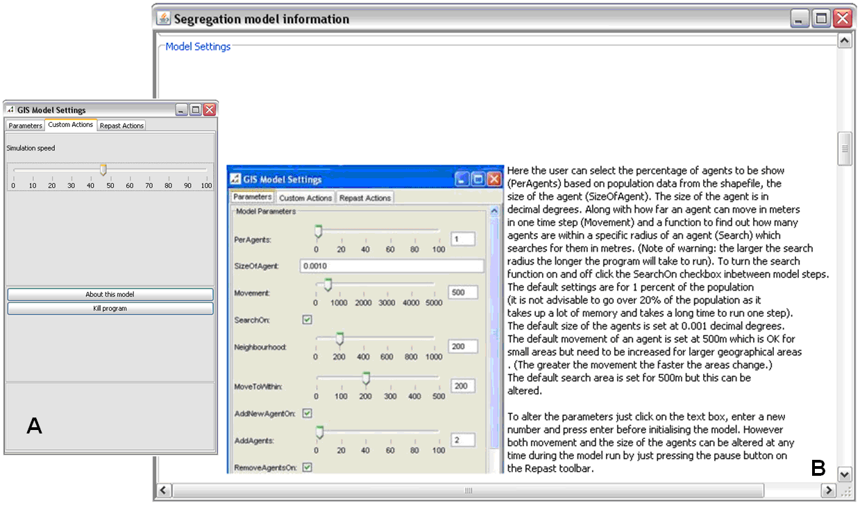
Figure 12: A: 'Custom Actions' pane which allows the user to see additional information about the model. B: additional information about the model.
Running the model
The previous sections have highlighted the core functionality of the basic model. This section describes briefly how the model is actually built. The model building process is broken down into a series of distinct parts, specifically, the build model/pre-running, and running phases of the simulation (Figure 13).
Figure 13: Basic Model Framework
The pre-running stage is composed of three main methods, that of buildModel, buildDisplay and buildSchedule, all of which are contained within the Basic Model class. A summary of the classes within the basic model is given below. This model class coordinates the setup and running of the model. The first task is to build the model. This is achieved through the buildModel method which defines the initial values to create the model; for example, the initial model parameters and the reading in the shapefiles which create the agents, be they polygons or points using data held in the rows and fields of the .dbf associated with the chosen shapefile. Agents are created by calling their respective classes, for example, polygon agent class or the point agent class which describes the behaviour of the specific agent being created. This information is passed back to the model class and stored as an ArrayList (a Java class that implements a dynamically expandable array of objects). Each class of agent has its own ArrayList which is a collection of objects (i.e. agents with their respective characteristics, for example, their co-ordinates, their income etc).
Once the agents have been created, the buildDisplay method is called which builds the GUI of the model. This includes the GIS viewer where each class of agent is added as a separate layer, for example, a polygon layer, and point agent layer and so forth based on information contained in their respective ArrayLists. Apart from the GIS display, there are also a series of methods which create a legend and graph displays. The graphs are used to chart the aggregate information of the model, for example, the type and number of agents which can change over time.
After the GUI of the model has been built, the final method that is called before starting the simulation is the buildSchedule. The buildSchedule method defines what actually happens during a simulation (i.e. at every time step) and in what order, therefore linking the pre-run and run phase of the model. The scheduling of events is broken down into three categories that of pre-Step, Step and post-Step. Events called in each of these methods are called sequentially; for example in one time step, first pre-Step will be called, and once all the actions have been done in pre-Step, Step is called and once all the actions have been done in Step, post-Step is called. Finally, once all the actions in post-Step have been executed, the time unit of the model advances by one. The reason for splitting time into three components is it separates the core behaviour of agent interaction in the Step method from the pre or post processing; for example, updating the display in pre-Step, if say the point agent has been moved by the user, and recording the change and updating the displays once all the agents have moved in post-Step. At this point, it is worth stressing that the model updates agents’ states asynchronously as each agent is updated one at a time; for example, one agent moves before another agent moves.
Below is summary of the classes within the basic model:
- BasicAgentArrayList: Takes a list of BasicPointAgents and sorts them into a list based on their Euclidian distance from the BasicPointAgent in question. Returns a list of agents with the nearest agent being returned first.
- BasicLine: Allows for the representation of ESRI Polylines. Records both the start and end node of each line and associated attribute information.
- BasicModel: Coordinates the setup and the execution of the model.
- BasicModelInfo: Creates a new window where information about the model can be displayed.
- BasicSmallNeighbourhoodArrayList: Sorts the BasicSmallNeighbourhoods-AttributesGeometry by a specific attribute. For example, accessibility which returns a list of small areas with the highest accessibility first.
- BasicSmallNeighbourhoodsAttributesGeometry: Stores the geometry and associated attributes of small neighbourhoods.
- BasicSmallNeighbourhoodsArrayList: Creates a series of small overlapping areas for the entire area which assist in the searching the BasicPointAgents use.
- BasicPoint: Allows point features from an ESRI point shapefile to be created and displayed within the model and then displayed.
- BasicPointAgents: point agents. Gives each point agent a location and other attributes such as a social class, age etc..
- BasicPolygonAgents: Creates the environment in which BasicPointAgents interact. Additionally contains methods that allow for point in polygon and union operations to be carried out.
- BasicStatistics: Allows for the calculation of certain statistics from an array of numbers such as maximum, mean, medium, quartiles, minimum, and sum.
- ShapefileChooser: Called from BasicModel when the model is first initialised. It allows the user to choose a shapefile for the model to be built upon.
Dynamics
As with agent characteristics, the dynamics within the model is entirely unspecified at the outset. The modeller can thus program dynamics into the model utilizing Repast’s scheduling mechanism, using the pre-Step, Step and post-Step methods. However, a specific time period can be considered such as a ‘second’ if the purpose is to model pedestrian movement, or ‘years’ for the residential dynamics. Additionally these different scales of dynamics can be incorporated into the same model if desired by using numerous internal clocks of agents. This was considered extremely important as different urban processes operate on different time scales. For example Liu and Andersson (2004) list three land-use change processes, slow, medium and fast. Slow processes are classed as those on a 3-5 year time scale, for example, as affecting the physical structure of the city (industrial, residential and transport construction). Medium time processes are classed as those relating to economic, demographic and several technological changes, which affect the usage of the physical structures and occur over months. Fast processes are classed as those that are less than one year often in months or weeks, such as the mobility of labour, goods and information. All three affect the location of both residents and businesses, and all could be represented within the agent-based model using a series of internal clocks.
Performance
It is not the intention of this paper to evaluate the performance of the simulation, as these ‘relatively hypothetical’ models do not need to operate in real time, unlike say pedestrian evacuation models. Methods within the model were built as efficiently as possible using functions that have been optimised by professional developers (such as classes from JTS). The model itself provides a series of reusable components as the model was built iteratively, and each component part was tested to ensure that it worked correctly (known as unit testing) in this respect helping with the verification of the model.
One disadvantage with this approach is that vector GIS operations are quite memory intensive, due to lists of geometries being created every time say a point agent moves, and this is caused specifically by the use of buffering to identify agents’ neighbours. The buffering mechanism used within the model is rather basic as it calculates a buffer around the desired agent and then queries the x and y attributes of all the agents to see if any of them are within the buffer. The burden can be reduced by simplifying the geometries of the shapes used within the model; for example, a square polygon composed of a thousand points takes longer to compare than a square polygon of four points.
Open questions for agent-based simulation focus on scale-up issues encountered in simulating large numbers of agents; specifically, ‘how many agents can be included in a workable agent-based simulation?’ (Macal and Howe, 2006) is an important issue. For this reason when the model is being built, the user has the option to create only a percentage of the actual population and thus the model can be run for a ‘sample’ of agents.
Summary of Basic Model
This page has presented the basic outline of an agent-based model utilising points, lines and polygons. This is a movement away from many of the current agent-based models utilizing GIS which are rooted in grid-based structures. Two main types of agents are described as polygons and points, both of which are spatially explicit. It is however the application which makes the model context-specific. For this reason there was no mention of agents’ behaviour. How agents’ behaviour is incorporated into the model will be explored in the subsequent pages where we adapt this framework to specific examples.
References
Barrett, C.L., Beckman, R.J., Berkbigler, K.P., Bisset, K.R., Bush, B.W., Campbell, K., Eubank, S., Henson, K.M., Hurford, J.M., Kubicek, D.A., Marathe, M.V., Romero, P.R., Smith, J.P., Smith, L.L., Stretz, P.E., Thayer, G.L., Van Eeckhout, E. and Williams, M.D. (2001), TRansportation ANalysis SIMulation System (TRANSIMS). Portland Study Reports 1, LA-UR-01-5711, Los Alamos National Laboratory, Los Alamos, NM, Available at
http://public.lanl.gov/bwb/do/1745e7424473e8068ef9240364490eb5.pdf.
Benenson, I. and Omer, I. (2003), 'High-Resolution Census Data: Simple Ways to Make Them Useful', Data Science Journal (Spatial Data Usability Special Section), 2: 117-127.
Benenson, I., Omer, I. and Hatna, E. (2002), 'Entity-Based Modelling of Urban Residential Dynamics: The Case of Yaffo, Tel Aviv', Environment and Planning B, 29(4): 491-512.
Liu, X. and Andersson, C. (2004), 'Assessing the Impact of Temporal Dynamics on Land-Use Change Modelling', Computers Environment and Urban Systems, 28(1-2): 107-124.
Lowry, I.S. (1965), 'A Short Course in Model Design', Journal of the American Institute of Planners, 31: 158-165.
Macal, C.M. and Howe, T.R. (2006), 'Who's Your Neighbour? Neighbour Identification for Agent-Based Modelling', in Sallach, D., Macal, C.M., and North, M.J. (eds.), Proceedings of the Agent 2006 Conference on Social Agents: Results and Prospects, University of Chicago and Argonne National Laboratory, Chicago, IL, Available at http://agent2007.anl.gov/2006procpdf/Agent_2006.pdf.
Najlis, R. and North, M.J. (2004), 'Repast for GIS', in Macal, C. M., Sallach, D. and North, M.J. (eds.), Proceedings of the Agent 2004 Conference on Social Dynamics: Interaction, Reflexivity and Emergence, Chicago, IL, pp. 255-260, Available at
http://www.agent2005.anl.gov/Agent2004.pdf.
Wilson, A.G. (2000), Complex Spatial Systems: The Modelling Foundations of Urban and Regional Analysis, Pearson Education, Harlow, UK